Hard Drive Selection for DVRs

This and the next few posts will be focusing on hard drive selection for DVRs. This post will look at the type of workload that a DVR imposes on drives, using Project Entangle as an example. Subsequent posts will look at various system characteristics that can affect performance and performance measurements from some drives. And we’ll take a special look at shingled magnetic recording (SMR) drives, as they tend to have some very peculiar performance characteristics.

The DVR Workload

Before we start looking at what metrics we might use to evaluate a drive, let’s take a look at the demands a DVR makes on one while recording and playing shows. Recording and playback are often characterized as “real-time” or time-critical operations – if the disk can’t keep up with the show as it comes in from the tuner, pieces of it will get dropped on the floor. And if it can’t be read off the disk in real-time then you’ll be staring at stalled video occasionally.

That’s not to say that DVRs don’t use disks for other purposes which are time critical in their own ways. For example they may employ databases to hold program guide data and store user interface elements on the disk. Slow access to these items could mean delays in bringing up a show’s description once you select it from a program guide, or screens may take a while to navigate to. Since these items directly affect the DVR’s responsiveness they are as time critical (and from a user’s standpoint can be more time critical) than the recording workload.

Fortunately these non-recording/playback tasks are also the type that hard drive vendors attempt to optimize their disks for. The recording and playback workload on the other hand tends to be a bit outside the mainstream so drives may not be optimized for them. So in this post and the ones that follow we’re going to look at which drives make good candidates for recording and playback.

For the sake of brevity, we’ll call the drive where shows are recording and played from the media drive and the drive which holds the operating system, DVR software, databases, and other items the system drive. 

It should be noted that the best choice for the media drive may not make the best system drive. Arguably it wouldn’t be a bad idea to use separate drives for the two. For example you could use an SSD for the system drive, even though an SSD would make a questionable choice for the media drive.

Recording to SSDs?

The following discussion is focused on using hard drives rather than SSDs. I’m sure many of you are tempted to use SSDs, and depending on how many shows you intend to record it may indeed be a very viable solution.

However SSD write endurance, particularly for the media drive, is something that should be kept in mind. This post discusses the caveats in more detail.

The Recording Workload

As mentioned above, recording is typically viewed as a critical real-time task. But while recording is the “R” in DVR, it’s also a somewhat behind-the-scenes activity. Users don’t interact with the recording process and aren’t affected by how fast a chunk of a show is written to disk – unless of course the disk is so slow that bits and pieces of your shows ends up being dropped on the floor.

Recording multiple channels

To get an idea of the DVR recording workload, let’s take a look at what we’re asking it to do. Your DVR is typically recording several shows at once, limited by the number of tuners it has. In a dual-tuner DVR you could record two shows simultaneously, while with an eight-tuner DVR you could be recording eight shows. Keep in mind that the DVR could be recording a show even if you didn’t ask to record anything. It could use a recommendation engine to record shows it thinks you might want. Or it could maintain a live cache, as TiVos do.

It’s also possible that you could “record” from sources other than a tuner. For example you could download a show from a content service or transfer a show from another device. These non-tuner “recordings” don’t have any real-time requirements – if the DVR decides to slow down the rate it writes them to disk, nothing will be lost. They could be handled on a best-effort basis. Unless of course you’re watching it as its being downloaded. In that case the download must occur in realtime. For the sake of modelling – and in the event that you are watching the show as its being downloaded – we’re going to treat these non-tuner recordings the same as tuner-based recordings.

Recording Bitrate

Whether we’re recording from a tuner or some other source, the show being recorded is providing bits at a certain rate. For over-the-air ATSC in the US, that can be as high as 19.39 Mbit/s. Those bits can be buffered for a while, but there’s only so much RAM available to cache things before those bits need to make their way onto the hard drive. If the internal buffers overflow because the drive is too slow, then pieces of the show get lost. While the DVR shouldn’t crash, when you get around to watching the show parts of it will be missing (inevitably they will be plot-critical), and you’ll see ugly blocking around the missing segments.

As a concrete example, say we’re recording eight shows simultaneously (on ABC, NBC, CBS, FOX, CW, PBS, and a couple other stations). While we might not be recording eight shows all the time, it’s quite possible that this will happen during primetime TV hours. Let’s also assume each of these channels is broadcast at the full 19.39 Mbit/s.

The aggregate bitrate of the eight channels is 19.39 Mbit/s * 8 = 18.49 MiB/s. (For clarity, this post uses kibibytes/kibibits/mibibytes/mibibits power-of-two units where appropriate. While the M and K prefixes denote 1,000,000 and 1,000 respectively, the Mi and Ki prefixes denote 1,048,576 and 1024 respectively.)

Subchannel Bitrates

Now you might question why were using the full 19.39 Mbit/s in our calculations. After all it’s common for multiple channels get crammed into that 19.39 Mbit/s. For example, in the San Francisco Bay Area the local ABC affiliate KGO broadcasts as 7-1. Alongside it in the same 19.39 Mbit/s stream is 7-2 (Live Well Network) and 7-3 (Laff). The bits tend to get divided between the channels as follows:

VC	Station	Average Bitrate (Mbit/s)	Video Format
7-1	KGO	11.05728	1280x720p@59.94
7-2	Live Well	6.03456	1280x720p@59.94
7-3	Laff	1.97952	704x480i@29.97
PSIP		0.094080
NULL (padding)		0.032640

As you can see, most of the bits go to the 720p KGO broadcast, but a good fraction of the 19.39 Mbit/s goes to the other channels.

Since 7-1 only uses 11.1 Mbit/s, it would be tempting to use something other than 19.39 Mbit/s in computing the recording and playback workload. For example 13 Mbit/s would more or less match the average bitrate of HD channels in the SF Bay Area. However given that you don’t know which set of channels you’re going to be recording at a time (and really don’t want to worry about that) there’s no safe bitrate less than 19.39 Mbit/s. While 7-1 only uses 11.1 Mbit/s, take a look at the CW affiliate 44-1.

VC	Station	Average Bitrate (Mbit/s)	Video Format
44-1	KBCW	15.42589	1920x1080i@29.97
PSIP		0.142187
NULL (padding)		3.631922

As it turns out 44-1 doesn’t share its bandwidth with anyone – it has the entire 19.39 Mbit/s to itself. And to make things even more convoluted, broadcasters can change the allocation of bits to channels over time, and even throughout a day.

For those reasons, we’re going to take a conservative approach and assume that each channel uses the full 19.39 Mbit/s.

Random Access Writes

Any modern hard drive can sustain 18.49 MiB/s as sequential writes. But we would only be writing sequentially if we were storing all eight shows interleaved in a single file. That’s generally not practical (and would  be something of a headache during playback, or when you wanted to delete a show). In addition, as you delete shows the free space becomes fragmented. So in practice those 18.49 MiB/s of writes will be scattered across the disk.

Random access in hard drives is quite expensive due to the time it takes to move the drive heads. We’ll examine exactly how much a penalty is incurred shortly. But for now let’s get a handle on how fragmented the writes may be. The filesystem’s allocation unit and the DVR’s I/O size are two factors that influence how contiguous the writes end up.

File system Allocation Unit

While performance metrics are often taken on a bare disk, in reality we don’t record or play back shows quite that way. The recorded shows are stored in a filesystem – whether a standard, general-purpose filesystem such as ext4 or NTFS, or a custom filesystem such as TiVo’s Media Filesystem. Either way, the filesystem breaks the disk up into blocks, and each file consists of one or more blocks.  A block is a contiguous area on disk and usually the smallest unit that can be allocated. Large block sizes improve performance since they encourage sequential reads and writes. However a large block size also could mean lots of wasted space – storing ten bytes in a 1 MiB block means you’ve wasted most of that 1 MiB.

Large block sizes are ideal for filesystems that will be holding recorded shows. Even at a data rate of 2 Mbit/s, which some SD channels may use, a half hour show is 450 MB. So from that perspective 16 MiB or even 128 MiB block sizes wouldn’t be a bad idea. Sadly, existing Linux filesystems don’t allow you to specify such large block sizes. Many filesystems constrain you to 4KiB, and even the xfs filesystem only gets you to 64 KiB. The ext4 filesystem does have the bigalloc feature, which through some sleight of hand allows clusters of blocks to be used as the allocation unit rather than individual blocks. The bigalloc feature allows allocation units to grow into the megabytes. Unfortunately support for bigalloc isn’t universal – for example it’s not supported in Centos/RHEL 7.4.

While we can’t use large allocation units, filesystems have other features which attempt to ensure  consecutive parts of a file are laid out in  consecutive sectors on the disk. ext4 uses extents, for example. Entangle uses ext4, and when I took a look at the files to store recordings, the vast majority (>99.9%) of extents were 1024 blocks (4 MiB) or larger.

So it wouldn’t be unreasonable to assume, at least from a filesystem standpoint, that we can read or write 4 MiB sequentially to the disk.

DVR I/O Size

While large allocation units at the filesystem level lay the foundation for sequential I/O, the DVR software needs to take advantage of that by issuing large reads and writes.

Let’s say our DVR writes media to disk in 512KiB chunks. So we have 18.49 MiB / 512KiB = 37 chunks/s. Another way to look at it is that each 19.39 Mbit/s channel will generate one chunk every fifth of a second or so.

Let’s also assume that if we’re recording eight shows simultaneously, each is going into its own file. So every fifth of a second a 512 KiB block would be written for each of those eight channels. And we have no guarantee of where on the disk the space for the files was allocated. In the worst case, those eight writes will span the entire disk.

Good DVR software will attempt to adapt their writes to the throughput of the disk. For example, Entangle will coalesce 512 KiB chunks into 1024 KiB (or larger) chunks if it notices that chunks are queueing up. However for the sake of modeling the hard drive, it’s useful to ignore those optimizations.

RANDOM ACCCESS WRITE Requirement

As mentioned previously, slow or late writes don’t affect the user experience. We just don’t want to exhaust the buffer we’ve set aside to hold the media data as it’s on its way to the disk. Since RAM isn’t infinite, let’s say we have five seconds of buffer, or close to 100 MiB. Then the record workload for an eight-tuner DVR using 512 KiB writes is:

The Playback Workload

At some point you’re probably going to watch some of those shows that got recorded. For broadcast TV, a majority of the time is spent watching the show linearly. But periodically you’ll want to fast-forwarding over commercial breaks or do an instant replay.

I/O Latency

For recording, we said we didn’t really care how quickly the drive got around to writing our chunks to disk. We graciously set the limit at five seconds. But for playback, how quickly the hard drive responds  directly affects the user experience. When you press play, you want the show to start playing as soon as possible. You don’t want to wait for (or care about) other things that the drive may be working on. You certainly don’t want to wait five seconds.

Guaranteed data rate

In addition to responding quickly to user actions, the drive needs to sustain the bitrate for the recording that’s being played. This is usually not a large amount – 2 MiB/s or so. However, it needs to be maintained. The drive can’t go out to lunch for a minute and burst 120 MiB later. More than likely, if that were to happen you’d be staring at stalled video for a good part of a minute. And you don’t care that the 120 MiB arrived later. It wasn’t there when you wanted it.

In addition to sustaining the show’s nominal bitrate, if you want to do a 1.2x or 1.5x fast forward then the show needs to be read from disk at that rate. (For these trick modes every picture in the stream gets decoded, and select pictures are dropped. So the decoder gets stressed as well. This is required due to the properties of MPEG-2 and H.264/H.265 video, which aren’t really tailored for such fine-grained random access.)

Random Access Performance

When you get to fast-forward speeds beyond 3x or reverse playback, the DVR typically doesn’t read the show from the disk at a faster rate. While this may be ok for 1.5x or 3x playback, at 20x or 40x you’d be taxing the disk quite a bit! Instead, the DVR typically will jump around and read only those frames it wants to display. Let’s say at 40x fast-forward mode you want to display 6 frames each second. That means every sixth of a second we’re going to be seeking ahead in the show (by about 6.5s in this example) and pulling out a frame. And we want to be guaranteed a frame every sixth of a second so we have a smooth fast forward.

Playback performance requirements

Taken together, for playback we want low latency random-access reads with a minimum guaranteed data rate. But while there may be a large number of simultaneous shows being recorded (eight in the example above), the number of simultaneous playback sessions is generally smaller. One or two playbacks would meet the needs of most users.

For each playback we have two distinct workloads:

Additional Filesystem Workload

In addition to the reads and writes that the DVR software generates, the filesystem itself will generate additional reads and writes as part of its internal bookkeeping. These tend to be very small in comparison to the 512 KiB or 2 MiB I/Os that the DVR software are doing. However the time the drive spends handling these tasks will eat into the DVR read/write performance, and the cost of a seek is the same whether you end up reading or writing 1 byte or 1 MiB.

Measuring the filesystem overhead is beyond the scope of this post.  It would be a good idea to de-rate a drive’s performance by 10-15% to allow for filesystem overhead.

Measuring Hard Drive Performance

Now that we’ve had a look at how the DVR uses the hard drive, we can look at ways of measuring performance  to determine if a particular hard drive is suitable for a certain DVR configuration. By configuration we mean the number of simultaneous records and playbacks. A DVR that allows eight records and two playbacks places a far greater demand on the hard drive than one that does four records and one playback.

There are many ways one can go about determining a drive’s suitability. Here and in the following posts we’ll look at two:

Theoretical Analysis

As we’ve noted above, the DVR workload consists of a number of random access reads and writes. In our example we’ve used 512 KiB for records, 512 KiB for trick mode playback, and 2 MiB for non-trick mode playback.

We can determine how much each of these reads or writes will cost by looking at:

The access time itself is generally made up of a number of values such as seek time and rotational latency. Manufacturers often quote an average seek time. Depending on the particular manufacturer, this may be derived statistically by averaging over all possible seeks, or may simply be the time it takes for the head to travel a third of the disk. The rotational latency is how long it takes for the desired sector to appear under the head once the head reaches the right track. This depends on how fast the disk spins. Most consumer drives are in the range of 5200 RPM – 7200 RPM. On average, half of a rotation is required before the target sector is under the head.

Additional access time factors include the time it takes for the head to “settle” once it reaches the target track, and how long it takes for the drive to internally process the commands its been given. Both these values tend to be very small (on the order of microseconds).

To give you an idea of the relative contribution of these factors, let’s consider a 512 KiB read at the midpoint of a 5400 RPM disk. Assume we’ve just read from sector 0, so the drive head needs to seek half way across the disk. Also assume that at the midpoint of the disk the sequential transfer rate is 100 MiB/s.

As you can see, the actual data transfer time is dwarfed by the other factors. The total time to read 512 KiB is about 25.6 ms. Although the disk has a rather high sequential read rate of 100 MiB/s, the seek time and rotational latency significantly degrade the effective throughput (~20 MiB/s)

HDTune is a popular tool for measuring drive properties. The following shows the sequential write and access time for the Toshiba MQ03ABB300:

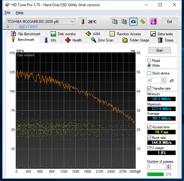
From the graph you can see that the sequential write performance varies from about 125 MiB/s at the outer tracks of the disk to around 60 MiB/s at the inner tracks. It’s typical that the read/write speed tends to decrease as you proceed along the drive. The reason is that sector 0 is on the outer track of the disk, while the last sector is on the innermost. If you visualize the circumference of these two tracks, you can see that the outer track’s circumference is quite larger than the inner track’s. Simply stated, that outer track can hold more bits. And since modern hard drives typically spin at the same rate regardless of where on the disk you’re reading or writing, the data rate tends to fall as you move from the outer tracks to the inner tracks.

The access time holds at a fairly constant 20 ms +/- 5ms. Note that HD Tune’s access time measurement is the time it takes to do a 64 KiB write, so includes seek time, rotational latency, and data transfer time.

The paid (Pro) version of HDTune also has a random access test:

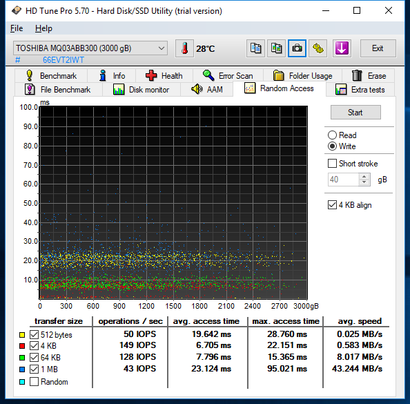
While it may not have the exact I/O size that your DVR uses (we’ve been using 512 KiB, which HDTune doesn’t measure), it does give you a way to sanity check the mathematical inferences. The 23.124 ms average access time for 1 MB transfers is in line with what you’d expect given the sequential write and 64 KiB access time numbers. What is also valuable is looking at the distribution of the access times, which range as high as 95 ms for 1 MiB writes. The majority of the access time cluster around 25 ms for 1 MiB, so it’s not something to be terribly worried about.

Caching, SMR, and Other Factors

So far it seems fairly straightforward to take metrics such as the drive’s access time and sequential read/write rates and get an idea of how suitable the drive  would be in a DVR. However things aren’t always so simple. In their quest to optimize performance or storage capacity drive manufacturers have introduced features that add a bit of non-determinism to the equation. And the operating system’s disk scheduler can throw a wrench into things too.

Shingled Magnetic Recording

Shingled magnetic recording (SMR) has gained some notoriety in recent years since it trades performance for capacity. In an SMR drive, the tracks are so close together that as a track is being written, data in adjacent tracks are disturbed. To guarantee the integrity of those tracks, they need to be rewritten. SMR drives are partitioned into zones. There’s space between zones so that writing to the last track in one zone doesn’t affect the first track in the next zone. However when you write any part of a zone, you need to rewrite the entire zone. So in order to write 4 KiB, you may end up writing many megabytes.

We’ll take a look at SMR in more detail, but for now I’d like to make clear one thing that seems to have a lot of people confused: SMR and PMR are complementary technologies. One way to think of it is PMR is the way the bits are laid out within a track. SMR is a way to pack those tracks closer together. So just because a drive says it uses PMR – and basically all current drives do – doesn’t mean it doesn’t also use SMR. And SMR as a method of increasing drive capacity is here to stay. Drive vendors have been fairly up-front that SMR will be used in conjunction with future technologies such as HAMR and MAMR. As is the case with PMR+SMR, the SMR variant of the HAMR or MAMR drives will have a higher capacity but incur the zone writing penalty. The non-SMR version will have more deterministic random write performance at thee expense of capacity.

Caching

All drives have some amount of volatile SRAM or DRAM-based high-speed cache. On the write side of things, caching means that the system can transfer data to the cache and then go on to do more things without waiting for the data to be transferred to the spinning media itself. This sounds great, except of course that until the data has hit the spinning media it could be lost. So if critical data is being written to the disk, it is necessary to wait until the drive signals that the data has made its way out of the cache onto the spinning media. But what if there were a bunch of writes queued up the cache? Well, you could end up waiting for quite a while as all those previous writes get sent to the spinning media. So write caching can overall benefit performance, but can also make performance a bit non-deterministic.

On the read side of things, caching can also result in some non-determinism. Here it’s more the effect of things like prefetching that can have a negative effect on performance. Drives can be set to prefetch some amount of data into their caches. As an example, say the drive is asked to read from sector X to sector Y. It may prefetch sector Y+1…Y+n on the assumption that it’ll be asked for that data in the near future. Of course doing so takes some time, and that may end up delaying a pending read or write by a small amount. The drive may also guess incorrectly – maybe those extra sectors aren’t the ones that will be needed soon. Remember that even if you’re sequentially reading a file, that file’s fragments may be scattered across the disk. And of course maybe those sectors will be read soon, but not soon enough. Other reads or writes may cause those sectors to be discarded from the cache before they’re fetched.

Operating System Disk Scheduler

A final variable we’ll touch on here is on the operating system side of things. In any system there are many applications contending for access to the drive. Even within an application there may be many threads of execution vying to read or write. Our hypothetical DVR for example has one thread of execution for each record and one for each playback.

Someone has to arbitrate among all these requestors, and that someone is the disk I/O scheduler. The scheduler looks at all the requests from each thread of execution and attempts to order them in an optimal fashion for the disk. Some operating systems such as Linux allow you to choose which scheduler should be used with each disk. We’ll take a look at how these schedulers interact with the DVR workload in a future post.

It should be noted that the scheduler best suited to recording and playing back shows is probably not the best for disks that hold databases or user interface assets. This is another reason why it may be a good idea to dedicate a drive to recorded shows, and have the operating system, DVR software and other items on a separate disk.

Simulating the DVR Workload

While tools like HDTune allow you to get a fairly good handle on a drive’s suitability, there’s no substitute for attempting to simulate the workload. Especially when one considers the non-determinism that can be introduced by the I/O scheduler, caching, and other factors.

The simulation we’ll use is based on the Entangle workload and consists of the following:

The simulation can be run in two modes, depending on the information we’re looking for:

Coming Soon…

That’s it for this post. In a coming post we’ll look at a few drives to see how they fare, both on paper (sequential read/write performance, access times) as well as in a simulated load. In particular we’ll take a look at the Toshiba MQ03ABBA300, which appears to have become the drive of choice for TiVo Bolt users. Its also the preferred drive for Entangles. And we’ll look at the ST4000LM016, which has had a somewhat less successful run as hard drive in TiVo Bolts (and is banned from Entangles).